Covariance vs Correlation in PCA: What’s the Difference?

Principal Component Analysis can use either correlation or covariance matrices, but when should you use which? This post walks through the fundamental differences between these two approaches.

Photo by Colin Watts.

Introduction

Principal Component Analysis (PCA) is a linear dimensionality reduction technique that identifies orthogonal directions (principal components) in the data along which variance is maximized. It projects high-dimensional data into a lower-dimensional space while preserving as much variability (information) as possible. Mathematically, PCA solves an eigenvalue problem on the covariance (or correlation) matrix of the data. When performing PCA, one must decide whether to apply it to the covariance matrix or the correlation matrix. This decision affects how variables with different scales contribute to the principal components. This post offers a technical explanation with a mathematical derivation to show why the covariance matrix of standardized data equals the correlation matrix of the original data. We’ll back this up with an example in R.

Proof

Let \(\mathbf{X} \in \mathbb{R}^{n \times p}\) be a data matrix with \(n\) observations and \(p\) variables.

• \(\mu_j = \frac{1}{n} \sum_{i=1}^n X_{ij}\) is the sample mean of variable \(j\)
• \(\sigma_j = \sqrt{\frac{1}{n-1} \sum_{i=1}^n (X_{ij} - \mu_j)^2}\) is its sample standard deviation

The centered data matrix is \(\tilde{\mathbf{X}} = \mathbf{X} - \mathbf{1}_n \mu^T\) where \(\mu \in \mathbb{R}^p\) is the vector of column means.

The covariance matrix of \(\mathbf{X}\) is defined as:

\[ \textbf{Cov}(\mathbf{X}) = \frac{1}{n-1} \tilde{\mathbf{X}}^T \tilde{\mathbf{X}} \]

The standardized data (i.e., \(\mu = 0\), \(\sigma = 1\)) is given by:

\[ Z_{ij} = \frac{X_{ij} - \mu_j}{\sigma_j} = \frac{\tilde{\mathbf{X}}}{\sigma_j} \quad \text{or} \quad \mathbf{Z} = \tilde{\mathbf{X}} \mathbf{D}^{-1} \]

where \(\mathbf{D} = \text{diag}(\sigma_1, \dots, \sigma_p)\)

Then,

\[ \begin{align*} \textbf{Cov}(\mathbf{Z}) &= \frac{1}{n-1} \mathbf{Z}^T \mathbf{Z} \\ &= \frac{1}{n-1} \left[\tilde{\mathbf{X}} \mathbf{D}^{-1}\right]^T \tilde{\mathbf{X}} \mathbf{D}^{-1}\\ &= \mathbf{D}^{-1}\frac{1}{n-1}\tilde{\mathbf{X}}^T \tilde{\mathbf{X}} \mathbf{D}^{-1}\\ &= \mathbf{D}^{-1} \textbf{Cov}(\tilde{\mathbf{X}}) \mathbf{D}^{-1}\\ \end{align*} \]

Now, to compute the correlation matrix of \(\mathbf{X}\), we normalize each covariance term by the product of the standard deviations of variables \(i\) and \(j\):

\[ \begin{align*} \textbf{Cor}(\mathbf{X})_{ij} &= \frac{\textbf{Cov}(\tilde{\mathbf{X}})_{ij}}{\sigma_i\sigma_j} \\ &= \mathbf{D}^{-1} \textbf{Cov}(\tilde{\mathbf{X}}) \mathbf{D}^{-1} \end{align*} \]

Thus: \(\boxed{\textbf{Cov}(\mathbf{Z}) = \textbf{Cor}(\mathbf{X})} \quad \blacksquare\)

This demonstrates that standardizing the data transforms the covariance matrix into the correlation matrix of the original variables.

PCA seeks directions (\(\mathbf{v}\)) that maximize the variance of the projected data:

\[ \max_{\mathbf{v} \in \mathbb{R}^p} \quad \mathbf{v}^T \Sigma \mathbf{v} \quad \text{subject to } \|\mathbf{v}\| = 1 \]

If \(\Sigma\) is the covariance matrix of \(\mathbf{X}\), this favors variables with large variance. If \(\Sigma\) is the correlation matrix (i.e., the covariance of standardized \(\mathbf{X}\)), all variables contribute equally. Indeed, the fact that the covariance matrix is unbounded (and scale-dependent), while the correlation matrix is bounded, \([-1, 1]\), and scale-free, is a fundamental reason why correlation-based PCA is preferred when variables are measured on different scales or units.

Example

Simulate correlated variables with different scales:

ssh = suppressPackageStartupMessages
ssh(library(DT))
ssh(library(tidyverse))
ssh(library(FactoMineR))

data(diamonds, "ggplot2")

Standardize the data:

Z <- diamonds |> 
  select(where(is.numeric)) |> 
  scale()

Covariance matrix of the standardized data:

cov_std <- Z |> 
  cov() |>
  round(3)

cov_std |> datatable()

Correlation matrix of the raw data:

cor_raw <- diamonds |> 
  select(where(is.numeric)) |> 
  cor() |>
  round(3)

cor_raw |> datatable()

Are they equal?

all.equal(cov_std, cor_raw)  # Should return TRUE

[1] TRUE

Since the diamonds dataset contains variables with heterogeneous scales, we perform PCA on the correlation matrix by using standardized data \(Z\). In the FactoMineR::PCA() function, we set the scale.unit argument to FALSE because our input data has already been standardized.

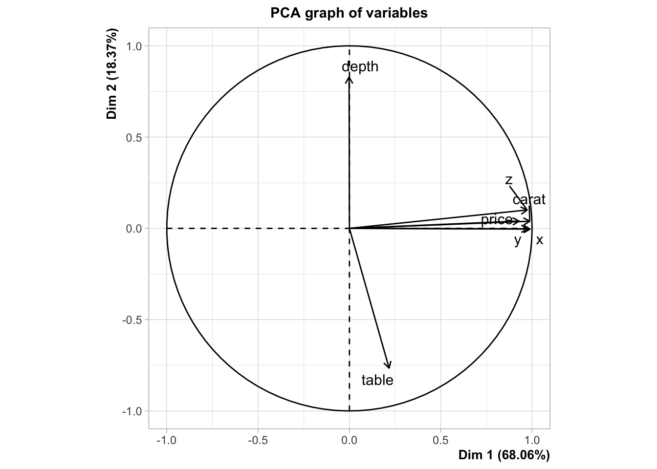
set.seed(123)
pca_mod <- PCA(Z, scale.unit = FALSE)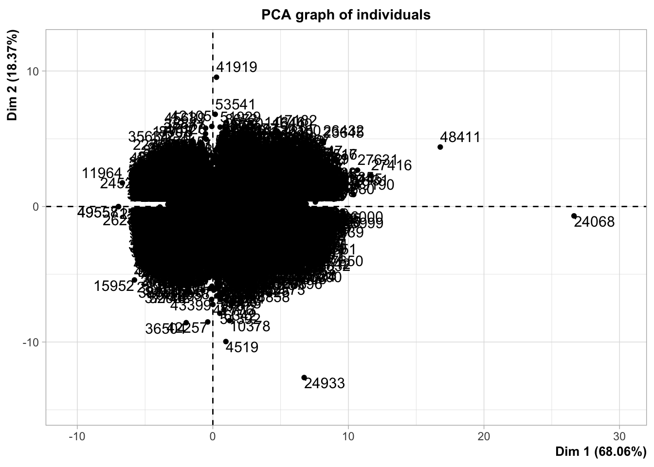

Conclusion

The covariance matrix of standardized data is mathematically equal to the correlation matrix of raw data. This equivalence means that applying PCA to standardized data is functionally identical to applying PCA directly to the correlation matrix of the raw data. This distinction is critical because the covariance matrix is scale-dependent and unbounded, which can cause variables with larger numerical ranges to dominate the principal components. In contrast, the correlation matrix is bounded between -1 and 1, ensuring that all variables contribute equally regardless of their original scale. Therefore, you must use correlation-based PCA, when your data consists of variables at different scales.