This function generates the adjusted boxplot, which is a robust graphical method for visualizing skewed data distributions. It provides a more accurate representation of the data's spread and skewness compared to standard boxplot, especially in the presence of outliers.
Usage
adjusted_boxplot(
  x,
  plot = TRUE,
  xlabels.angle = 90,
  xlabels.vjust = 1,
  xlabels.hjust = 1,
  box.width = 0.5,
  notch = FALSE,
  notchwidth = 0.5,
  staplewidth = 0.5
)
Arguments
- x
A numeric data frame or tibble.
- plot
A logical value indicating whether to plot the adjusted boxplot (default is
TRUE).- xlabels.angle
A numeric value specifying the angle (in degrees) for x-axis labels (default is 90).
- xlabels.vjust
A numeric value specifying the vertical justification of x-axis labels (default is 1).
- xlabels.hjust
A numeric value specifying the horizontal justification of x-axis labels (default is 1).
- box.width
A numeric value specifying the width of the boxplot (default is 0.5).
- notch
A logical value indicating whether to display a notched boxplot (default is
FALSE).- notchwidth
A numeric value specifying the width of the notch relative to the body of the boxplot (default is 0.5).
- staplewidth
A numeric value specifying the width of staples at the ends of the whiskers.
Value
If
plot = TRUE, returns aggplot2object containing the adjusted boxplot.If
plot = FALSE, returns a list of tibbles with the adjusted boxplot statistics and potantial outliers.
Details
The function is based on the medcouple (MC) measure computed on the data and which robustly measures skewness. This measure is bounded between −1 and 1. The medcouple is equal to zero when the observed distribution is symmetric, whereas a positive (resp. negative) value of MC corresponds to a right (resp. left) tailed distribution. It worth noting that this method is more appropriate for distributions that are not excessively skewed i.e., for \(|\text{MC}| \leq 0.6\).
References
The adjusted boxplot is based on the methodology described in:
Brys, G., Hubert, M., Struyf, A., (2004). A Robust Measure of Skewness. Journal of Computational and Graphical Statistics, 13(4):996-1017
Hubert, M., Vandervieren, E., (2008). An adjusted boxplot for skewed distributions. Computational Statistics and Data Analysis, 52(12):5186-5201
Examples
set.seed(123)
data <- data.frame(
normal = rnorm(100),
skewed = rexp(100, rate = 0.5),
heavy_tailed = rt(100, df = 3)
)
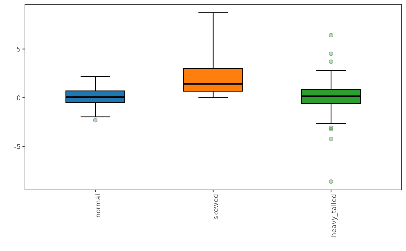
# Plot the adjusted boxplot
adjusted_boxplot(data)
#> The default of 'doScale' is FALSE now for stability;
#> set options(mc_doScale_quiet=TRUE) to suppress this (once per session) message
 # Retrieve the adjusted boxplot statistics
adjusted_boxplot(data, plot = FALSE)
#> $stats
#> # A tibble: 3 × 7
#> variable lower q1 median q3 upper medcouple
#> <fct> <dbl> <dbl> <dbl> <dbl> <dbl> <dbl>
#> 1 normal -1.97 -0.497 0.0618 0.695 2.19 0.0338
#> 2 skewed 0.00873 0.673 1.43 3.02 8.73 0.404
#> 3 heavy_tailed -2.63 -0.602 0.146 0.837 2.80 -0.0193
#>
#> $outliers
#> # A tibble: 8 × 2
#> variable value
#> <fct> <dbl>
#> 1 normal -2.31
#> 2 heavy_tailed 3.70
#> 3 heavy_tailed 6.42
#> 4 heavy_tailed -3.22
#> 5 heavy_tailed 4.51
#> 6 heavy_tailed -8.61
#> 7 heavy_tailed -3.09
#> 8 heavy_tailed -4.24
#>
# Retrieve the adjusted boxplot statistics
adjusted_boxplot(data, plot = FALSE)
#> $stats
#> # A tibble: 3 × 7
#> variable lower q1 median q3 upper medcouple
#> <fct> <dbl> <dbl> <dbl> <dbl> <dbl> <dbl>
#> 1 normal -1.97 -0.497 0.0618 0.695 2.19 0.0338
#> 2 skewed 0.00873 0.673 1.43 3.02 8.73 0.404
#> 3 heavy_tailed -2.63 -0.602 0.146 0.837 2.80 -0.0193
#>
#> $outliers
#> # A tibble: 8 × 2
#> variable value
#> <fct> <dbl>
#> 1 normal -2.31
#> 2 heavy_tailed 3.70
#> 3 heavy_tailed 6.42
#> 4 heavy_tailed -3.22
#> 5 heavy_tailed 4.51
#> 6 heavy_tailed -8.61
#> 7 heavy_tailed -3.09
#> 8 heavy_tailed -4.24
#>