Testing and experimenting.
The specProc package performs a wide range of preprocessing tasks essential for spectroscopic data analysis. Spectral preprocessing is essential in ensuring accurate and reliable results by minimizing the impact of various distortions and artifacts that can arise during data acquisition or due to inherent characteristics of the sample or instrument.
Some techniques are purely based on mathematical concepts, relying on robust statistics and signal processing techniques. Other methods are inspired by the physicochemical context of the dataset. These techniques rely on domain knowledge and exploit the fundamental principles governing the spectroscopic phenomenon used.
Installation
You can install the development version from GitHub with:
install.packages("devtools")
devtools::install_github("ChristianGoueguel/specProc")
Examples
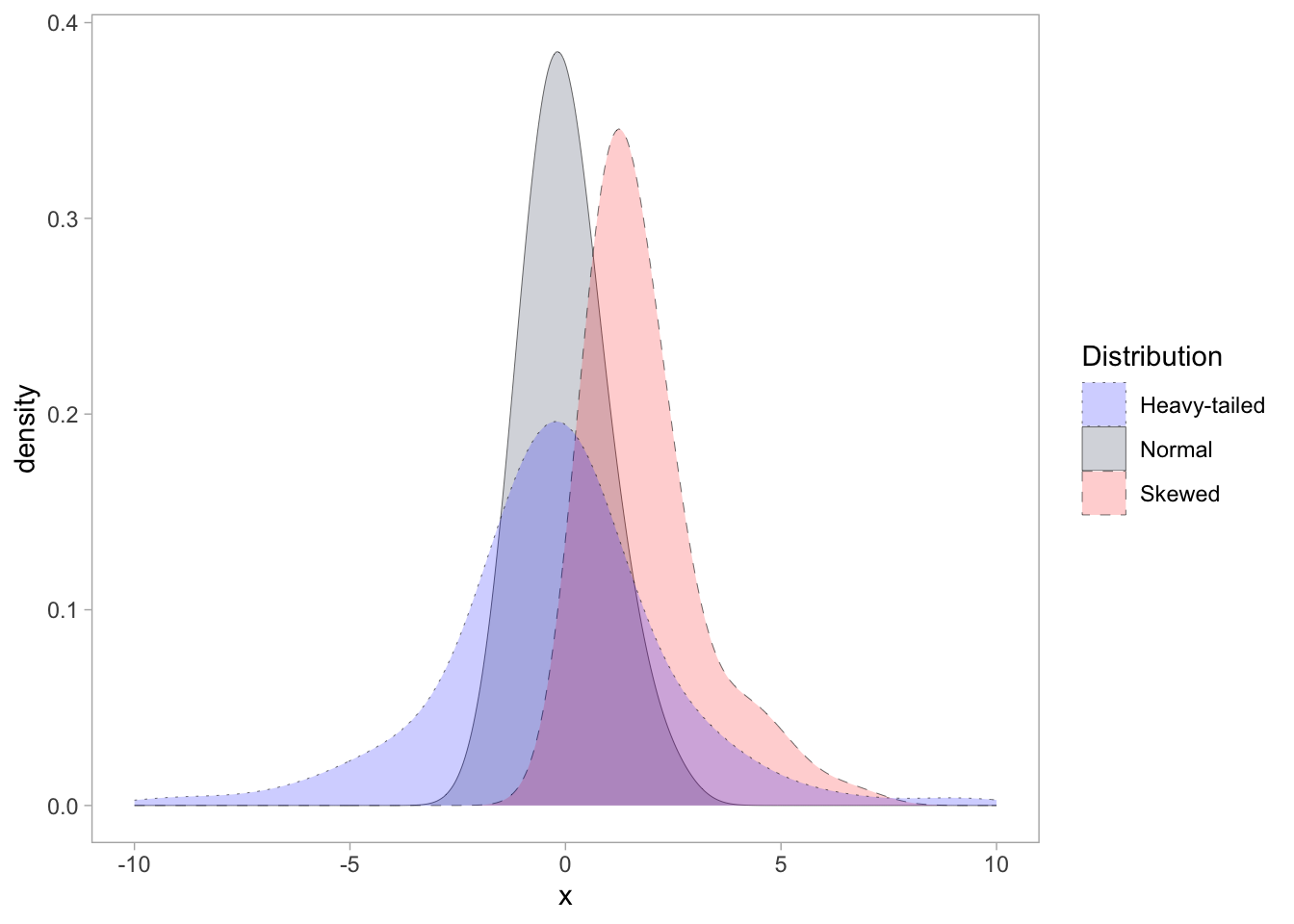
set.seed(02301)
tbl <- data.frame(
  normal = stats::rnorm(100),
  skewed = stats::rgamma(100, shape = 2, scale = 1),
  heavy_tailed = stats::rcauchy(100, location = 0, scale = 1)
  )
descriptive statistics
classical approach
specProc::summaryStats(tbl)
#> # A tibble: 3 × 14
#>   variable     mean  mode median   IQR    sd variance     cv     min   max range
#>   <chr>       <dbl> <dbl>  <dbl> <dbl> <dbl>    <dbl>  <dbl>   <dbl> <dbl> <dbl>
#> 1 heavy_tail…  0.44 -1.74  -0.22  2.36  6.54   42.7   1486.  -19.4   41.5  60.9
#> 2 normal       0    -0.4   -0.14  1.04  0.91    0.823 -Inf    -1.80   2.54  4.34
#> 3 skewed       1.83  6.82   1.37  1.32  1.32    1.73    72.1   0.160  6.82  6.66
#> # ℹ 3 more variables: skewness <dbl>, kurtosis <dbl>, count <int>
robust approach
specProc::summaryStats(tbl, robust = TRUE)
#> # A tibble: 3 × 14
#>   variable    median   mad    Qn    Sn medcouple   LMC   RMC   rsd biloc biscale
#>   <chr>        <dbl> <dbl> <dbl> <dbl>     <dbl> <dbl> <dbl> <dbl> <dbl>   <dbl>
#> 1 heavy_tail…  -0.22  1.74  2.2   2.03      0.1   0.35  0.63  2.58 -0.22    2.4
#> 2 normal       -0.14  0.82  0.92  0.93      0.19  0.29  0.55  1.22 -0.05    0.92
#> 3 skewed        1.37  0.95  0.91  0.85      0.46  0.2   0.43  1.41  1.58    1.18
#> # ℹ 3 more variables: bivar <dbl>, rcv <dbl>, count <int>
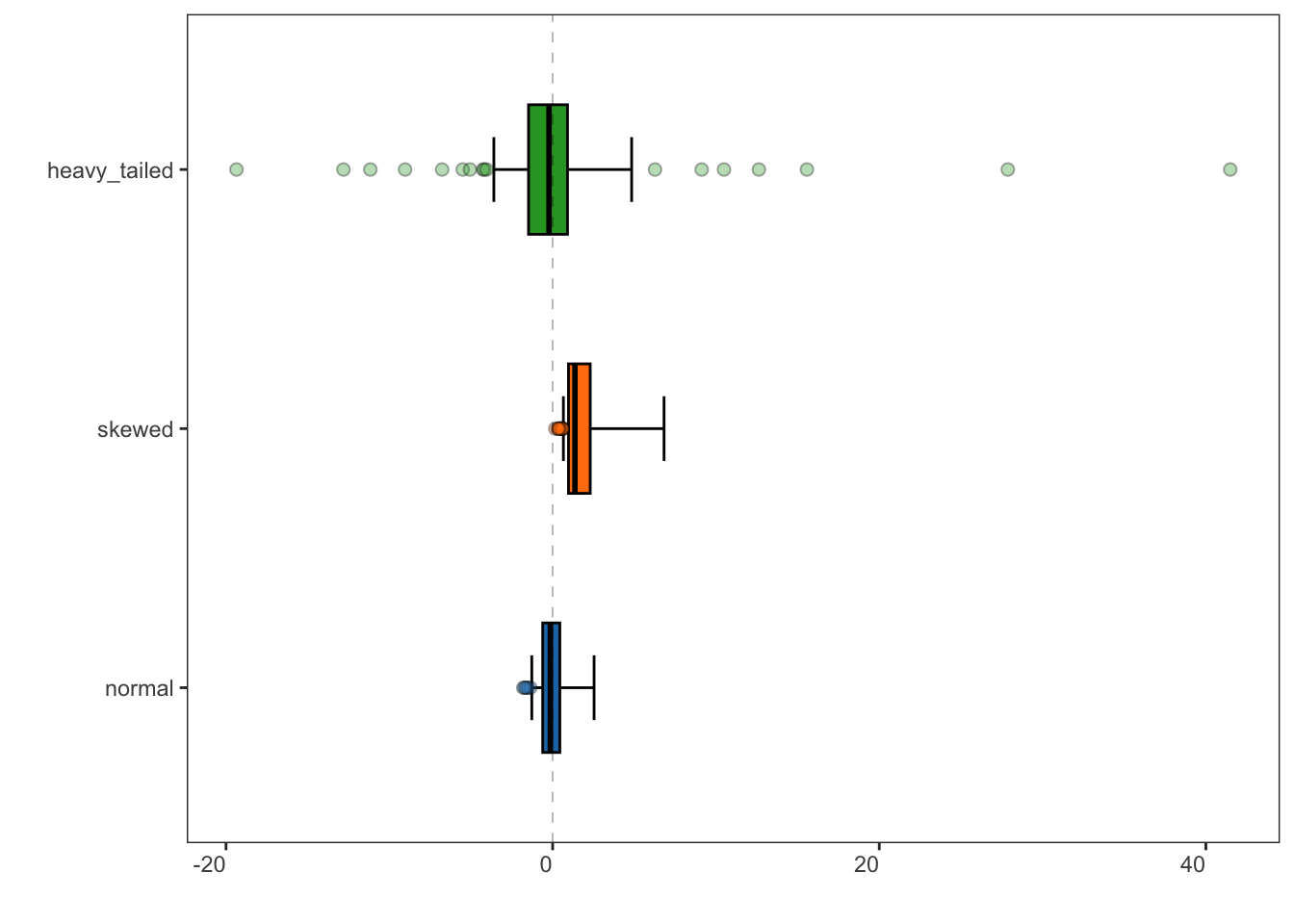
adjusted boxplot
specProc::adjusted_boxplot(tbl, xlabels.angle = 0) +
  ggplot2::geom_hline(yintercept = 0, linetype = "dashed", linewidth = 0.1) +
  ggplot2::coord_flip()
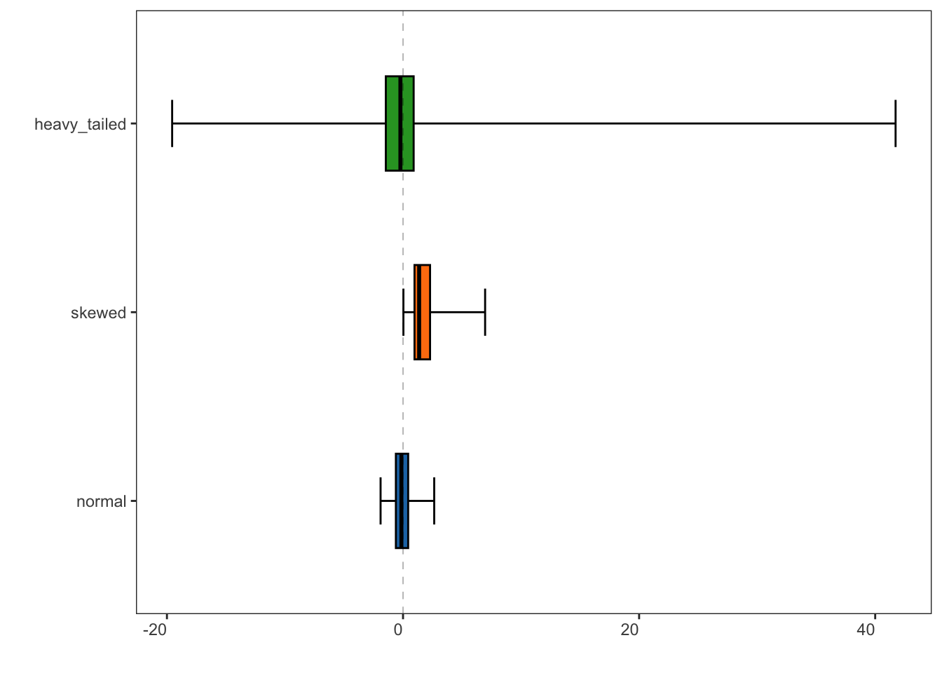
generalized boxplot
specProc::generalized_boxplot(tbl, xlabels.angle = 0) +
  ggplot2::geom_hline(yintercept = 0, linetype = "dashed", linewidth = 0.1) +
  ggplot2::coord_flip()
correlation
glass |> specProc::correlation(Na2O, method = "spearman", .plot = TRUE)
#> $correlation
#> # A tibble: 12 × 3
#>    variable .correlation method
#>    <chr>           <dbl> <chr>
#>  1 Cl              0.601 spearman
#>  2 SO3             0.406 spearman
#>  3 SiO2            0.244 spearman
#>  4 P2O5           -0.115 spearman
#>  5 BaO            -0.144 spearman
#>  6 MgO            -0.234 spearman
#>  7 MnO            -0.241 spearman
#>  8 Al2O3          -0.267 spearman
#>  9 Fe2O3          -0.281 spearman
#> 10 CaO            -0.316 spearman
#> 11 PbO            -0.356 spearman
#> 12 K2O            -0.571 spearman
#>
#> $plot


