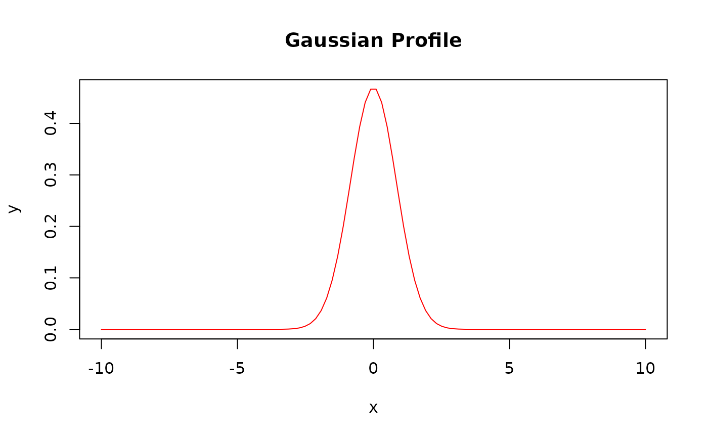
Computes the values of a Gaussian function (also known as the normal distribution) given specific parameters. The Gaussian profile is a bell-shaped curve that is symmetric around its center, making it distinct from other profiles like the Lorentzian profile, which has heavier tails.
Arguments
- x
A numeric vector representing the independent variable (e.g., wavelength, frequency).
- y0
A numeric value specifying the baseline offset.
- xc
A numeric value representing the center of the peak.
- wG
A numeric value specifying the full width at half maximum (FWHM).
- A
A numeric value representing the peak area.
Value
A numeric vector containing the values of the Gaussian function evaluated
at the provided x values.
Details
The Gaussian function is defined as:
$$y = y_{0} + \frac{A}{w_{G} \sqrt{\pi / (4 \log(2))}} \exp \left( -\frac{4 \log(2) (x - x_{c})^2}{w_{G}^2} \right)$$
where:
\(A\) is the peak area
\(x_c\) is the center of the peak
\(w_G\) is the full width at half maximum (FWHM)
\(y_0\) is the baseline offset
In spectroscopy, the Gaussian function is widely used to model the shape of spectral lines broadened by Doppler broadening, which arises from the thermal motion of atoms or molecules emitting or absorbing the radiation. However, in some cases, other broadening mechanisms, such as pressure broadening or natural broadening, may contribute to the overall line shape, leading to deviations from a pure Gaussian profile. In these situations, more complex line shape models, such as the Voigt profile (a convolution of Gaussian and Lorentzian profiles), may be required.
Additionally, instrumental broadening, caused by the finite resolution of the spectrometer or other experimental apparatus, is another important factor that can contribute to the observed spectral line shape, and it's often modeled using a Gaussian profile as well.