Lorentzian Function

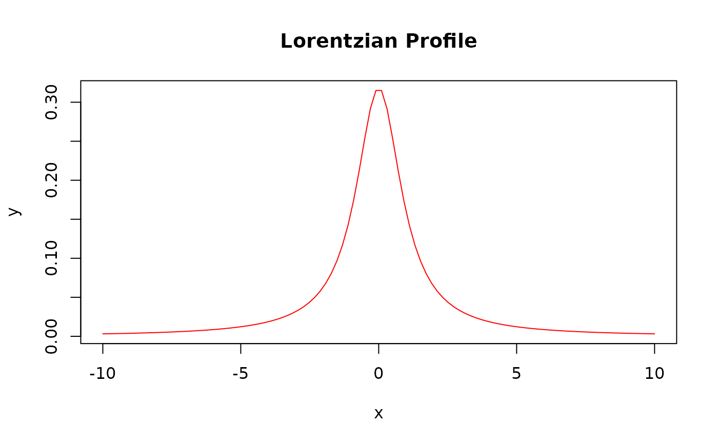
Computes the Lorentzian function, which is a peaked function with a distinctive bell-shaped curve and wider tails than the Gaussian function. The Lorentzian function is commonly used to model spectral line shapes.

Usage

lorentzian(x, y0, xc, wL, A)

Arguments

x

A numeric vector representing the independent variable (e.g., wavelength, frequency).

y0

A numeric value specifying the baseline offset.

xc

A numeric value representing the center of the peak.

wL

A numeric value specifying the full width at half maximum (FWHM).

A

A numeric value representing the peak area.

Value

A numeric vector containing the values of the Lorentzian function evaluated at the provided x values.

Details

The Lorentzian function is defined as:

$$y = y_{0} + \frac{A}{\pi} \frac{\gamma}{(x - x_c)^2 + \gamma^2}$$

where:

• \(A\) is the peak area

• \(x_c\) is the center of the peak

• \(\gamma = w_{L} / 2\) is the half-width at half maximum (HWHM)

• \(y_0\) is the baseline offset

The Lorentzian function arises naturally in various physical processes, such as the decay of excited states in atoms or molecules, and is commonly used to model phenomena that exhibit homogeneous broadening, where all atoms or molecules experience the same broadening mechanism.

Author

Christian L. Goueguel

Examples

x <- seq(-10, 10, length.out = 100)
y <- lorentzian(x, y0 = 0, xc = 0, wL = 2, A = 1)
plot(x, y, type = "l", col = "red", main = "Lorentzian Profile")