The Tukey g-and-h (TGH) distribution is a flexible family of parametric distributions that can accommodate a wide range of skewness and kurtosis values, making it useful for modeling non-normal data.
Usage
tukeyGH(
  x,
  type = "d",
  location = 0,
  scale = 1,
  g = 0,
  h = 0,
  log = FALSE,
  log.p = FALSE,
  n = NULL
)
Arguments
- x
A numeric vector or a single value, depending on the function being called.
- type
A character string specifying the function to be called (
dfor density,pfor cumulative distribution,qfor quantile, orrfor random number generation).- location
The location parameter of the TGH distribution.
- scale
The scale parameter of the TGH distribution.
- g
The skewness parameter of the TGH distribution.
- h
The kurtosis parameter of the TGH distribution.
- log
If
TRUE, the log-density is returned for the density function. Default isFALSE.- log.p
If
TRUE, the log-probability is returned for the cumulative distribution and quantile functions. Default isFALSE.- n
For random number generation, the number of random values to be generated. Default is
NULL.
Details
The Tukey g-and-h distribution, introduced by John W. Tukey in 1977, is defined by two transformation functions, g and h, which are applied to a standard normal distribution. The g transformation controls the skewness of the distribution, while the h transformation controls the kurtosis (or heaviness of the tails). The TGH distribution is given by:
$$T_{g,h}(Z) = \frac{1}{g} (e^{g Z} -1) e^{\frac{1}{2} h Z^2}$$
Where \(Z\) is a random variable with standard normal distribution. The parameters \(g\) and \(h\) stand for the bias and elongation of the tails, respectively, of Tukey’s \(g\)-and-\(h\) distribution.
References
Tukey, J.W., (1977). Modern techniques in data analysis. NSF‐sponsored regional research conference at Southeastern Massachusetts University, North Dartmouth, MA.
Martinez, J., Iglewicz, B., (1984). Some properties of the Tukey g and h family of distributions. Communications in Statistics: Theory and Methods, 13(3):353–369.
Hoaglin, D.C., (1985). Summarizing shape numerically: The g-and-h distributions. In: Hoaglin, D.C., Mosteller, F., Tukey, J.W., (eds), Data Analysis for Tables, Trends, and Shapes. New York:Wiley.
Examples
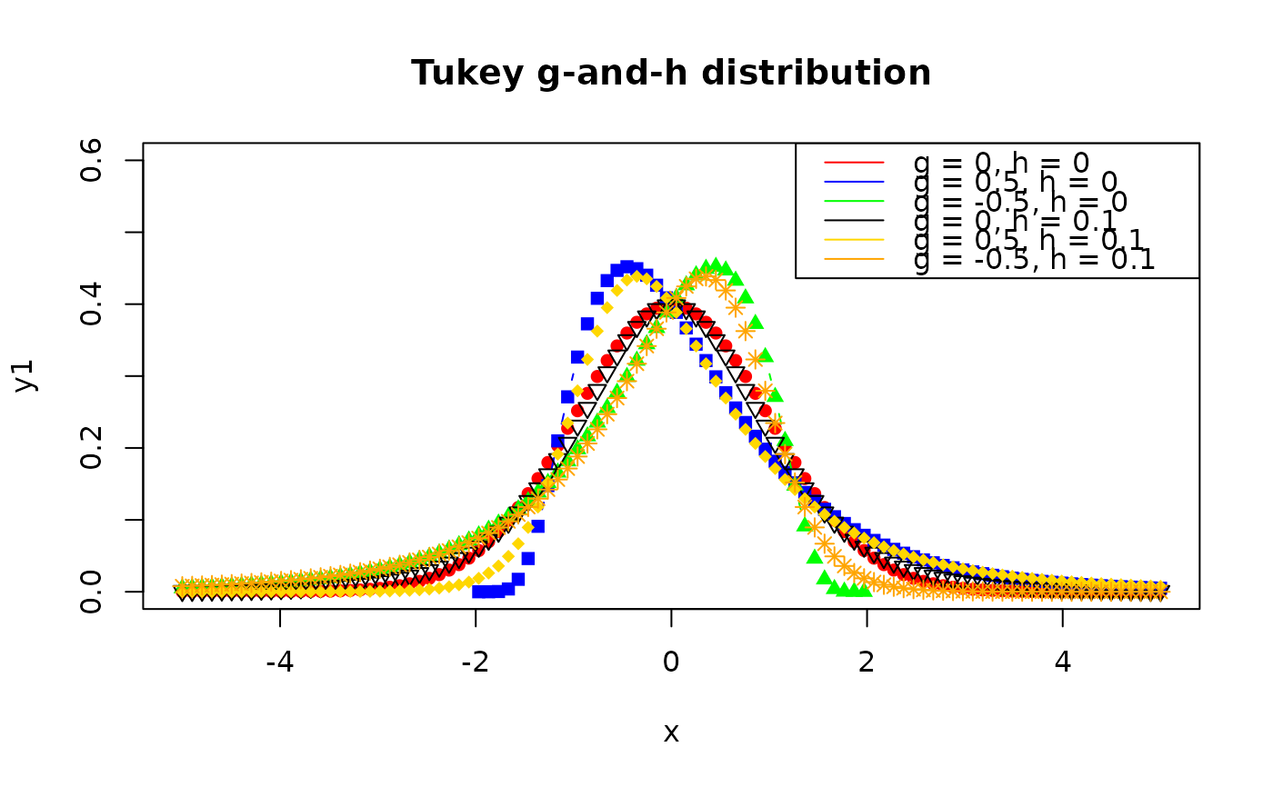
x <- seq(-5, 5, length.out = 100)
y1 <- tukeyGH(x, type = "d", location = 0, scale = 1, g = 0, h = 0)
y2 <- tukeyGH(x, type = "d", location = 0, scale = 1, g = 0.5, h = 0)
y3 <- tukeyGH(x, type = "d", location = 0, scale = 1, g = -0.5, h = 0)
y4 <- tukeyGH(x, type = "d", location = 0, scale = 1, g = 0, h = 0.1)
y5 <- tukeyGH(x, type = "d", location = 0, scale = 1, g = 0.5, h = 0.1)
y6 <- tukeyGH(x, type = "d", location = 0, scale = 1, g = -0.5, h = 0.1)
plot(x, y1, type = "b", col = "red", pch = 16,
main = "Tukey g-and-h distribution", ylim = c(0, 0.6))
lines(x, y2, type = "b", col = "blue", pch = 15)
lines(x, y3, type = "b", col = "green", pch = 17)
lines(x, y4, type = "b", col = "black", pch = 6)
lines(x, y5, type = "b", col = "gold", pch = 18)
lines(x, y6, type = "b", col = "orange", pch = 8)
legend(
"topright",
legend = c(
"g = 0, h = 0", "g = 0.5, h = 0", "g = -0.5, h = 0",
"g = 0, h = 0.1", "g = 0.5, h = 0.1", "g = -0.5, h = 0.1"),
col = c("red", "blue", "green", "black", "gold", "orange"),
lty = 1
)